Published September 2025 as part of the proceedings of the first Alpaca conference on Algorithmic Patterns in the Creative Arts, according to the Creative Commons Attribution license. Copyright remains with the authors.
doi:10.5281/zenodo.17084420
In this paper we handle pattern generation with a combinatorial approach by framing permutations as numeric literals. We highlight the advantages and limits of this notation to generate and index patterns. We show that this notation is robust, accessible, and tightly linked to existing mathematics, rendering the method universally available in programming languages. This approach allows the users to group the enumerated elements into consistent sets, enabling efficient creation, classification and analysis of patterns. We demonstrate the versatility of this approach with the Chicken Counter1, named with a play on the old proverb: “don’t count your chickens before they hatch”. It is a web app for visual, pixel-based-pattern exploration and can be considered as an accessible application of our flexible and extensible method. Our aim is to facilitate the application of a combinatorial approach based on the 18th century works of Sebastien Truchet (1704) and Dominique Doüat (1722) extending it within digital environments, scaling the potential of their method and improving the accessibility for computational exploration and creative practices.
The pattern generation method that we present is grounded on the works of Sebastien Truchet2 and Dominique Doüat3 dated 1704 and 1722 respectively.
The bright intuition of Sebastien Truchet was really simple: to apply a combinatorial study to a tiling module, in order to make its aesthetic potential emerge before starting to compose (fig. 1,2).
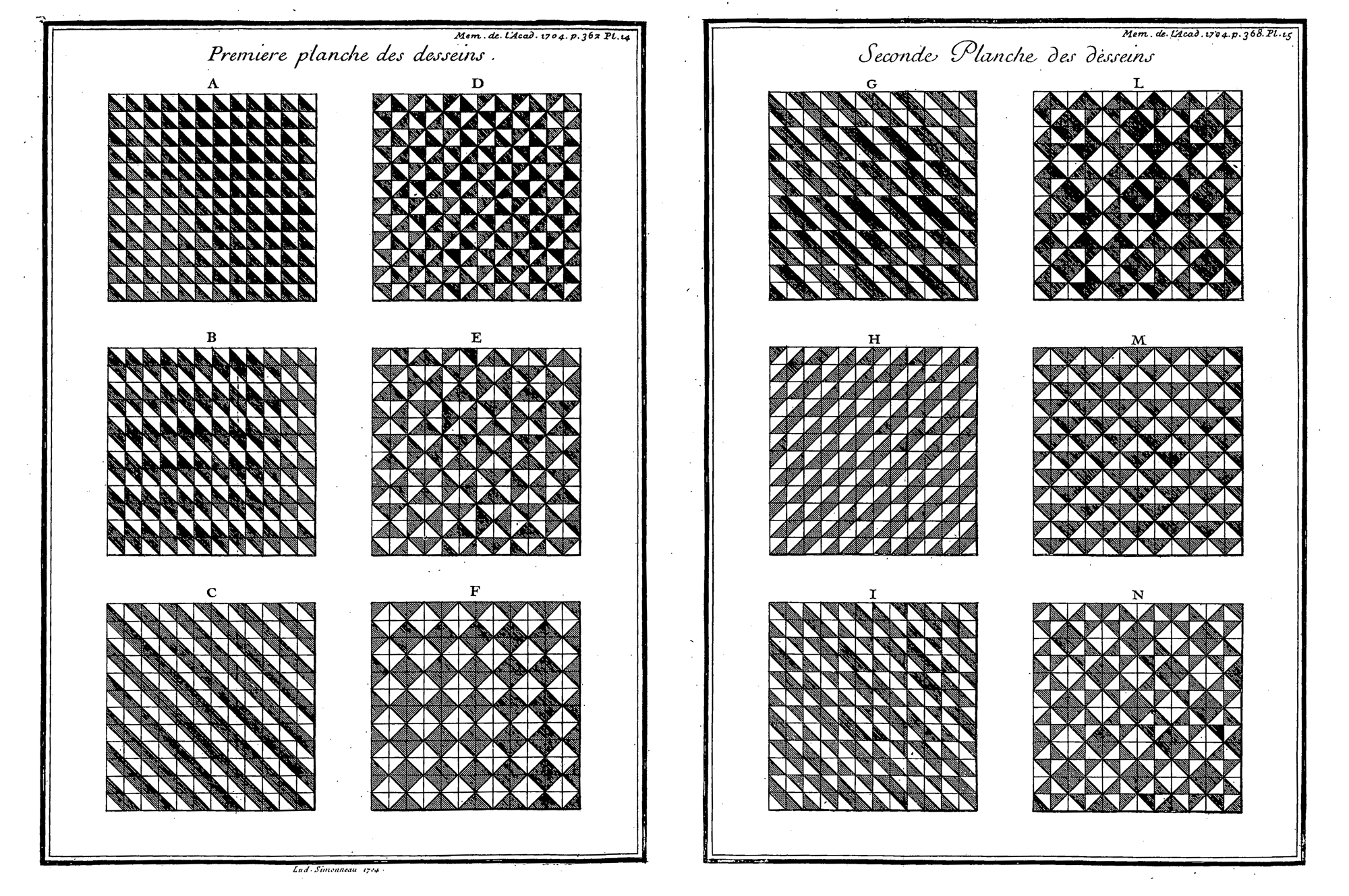
We can sum up his approach in four passages: 1. Define the initial modules (fig. 1, Table I). 2. Combine the modules in all possible permutations (Table I). 3. Create an ordered index of the permutations based on their visual appearance (fig. 2 Tables II and III). 4. Generate compositions by selecting permutations from the ordered index (fig. 2, Planches des desseins).
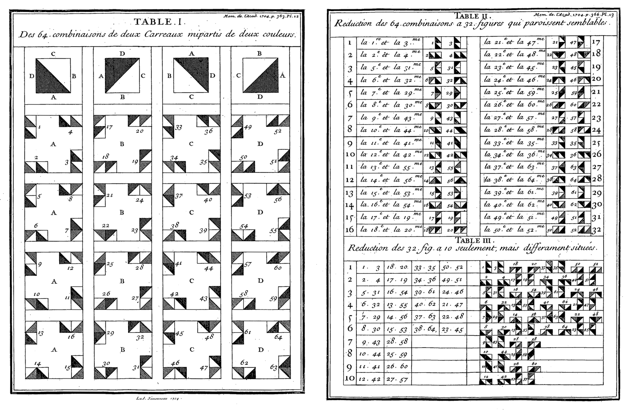
Dominique Doüat improved on Truchet’s approach introducing a new notation and calculation method for pattern generation, this made the manual work faster and more accurate.
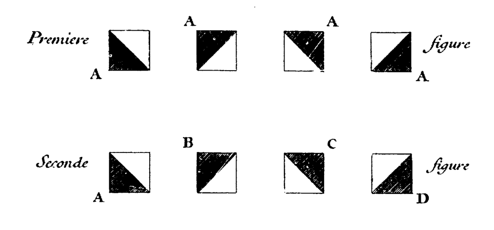
First, he associates a letter to every spatial configuration of the square module: A, B, C, D (fig. 3). Then, he combines elements 4 by 4 rather than in groups of 2, allowing the system to scale up better and let the aesthetic potential emerge.
In Doüat words:
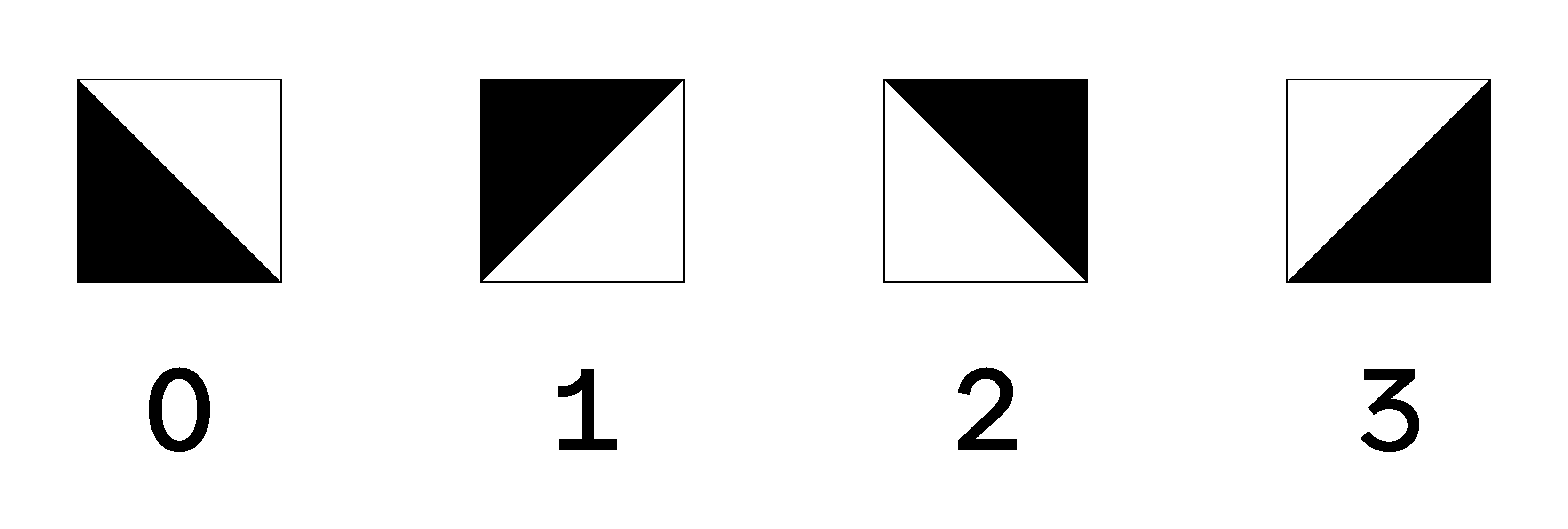
II. Observation The same tile A, when placed in different positions and viewed from the same side, can be considered as four different tiles: this is clear. We will call tile A the one with the colored corner at the bottom left; tile B, the one with the colored corner at the top left; tile C, the one with the colored corner at the top right; and tile D, the one with the colored corner at the bottom right. See (Figure 3, first row)
III. Observation The tiles A, B, C, D, when compared with one another, are opposed in three different ways: diagonally, horizontally, and perpendicularly. The tiles A & C, or C & A, B & D, or D & B, are opposed diagonally, that is, from white to black, or from black to white. The tiles A & D, or D & A, B & C, or C & B, are opposed horizontally, that is, from right to left, or from left to right. The tiles A & B, or B & A, C & D, or D & C, are opposed perpendicularly, that is, from top to bottom, or from bottom to top. It is clear, from the mere aspect of the four tiles figured hereafter. See (Figure 3, second row). Dominique Doüat, Methode pour faire un’infinité des Desseins […], Paris, 1722. Freely translated by the authors, see original4
Since the appearance and the reciprocal geometric properties of the modules has already been defined, Doüat’s notation made the method more efficient and created a “virtual” environment, where one could calculate combinations or notate pleasing visual compositions simply by writing (fig. 4), without even looking at the actual representation.
(Doüat also defined the rules for the catalogation of the obtained permutations, and some generative rules to compose with his notation.)
The main merit of Dominique Doüat is in understanding the power of notation for pattern generation.
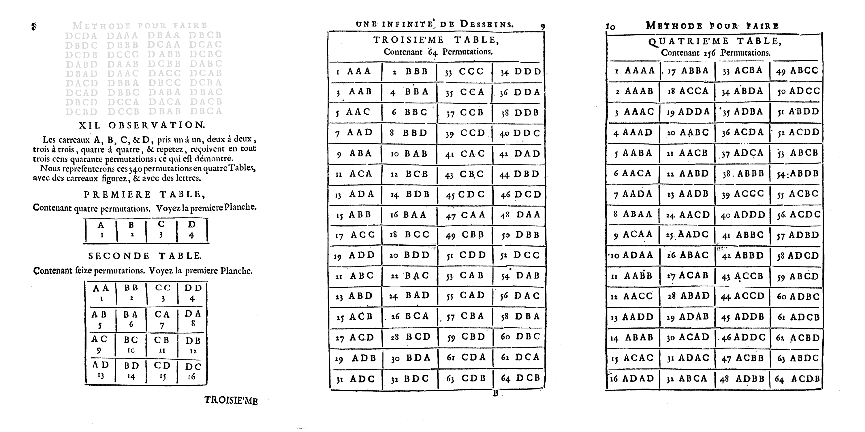
Doüat furthermore calculates the total possible compositions in a given space (fig. 5) and defines some generative rules for the composition of drawings5.
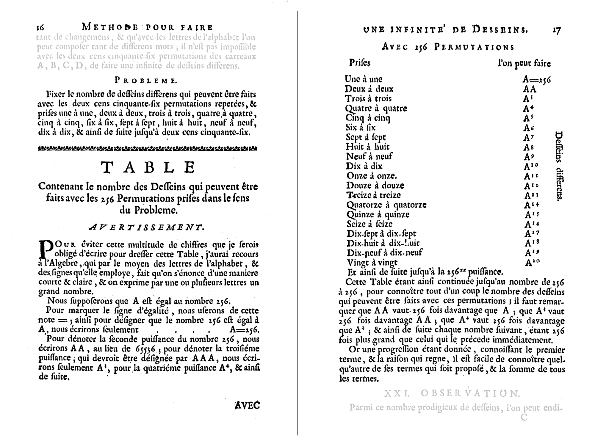
\(TotalCount = n^k\)
\(n\) : number of modules
\(k\) : class of the permutation
To conclude, the main difference between the work of Truchet and Douat is the notation: while the first was permutating tiles with a graphical notation, Douat was doing it tipographically, playing with strings.
The modular approach has already been recognized as a central strategy in contemporary design practice. As Martin Lorenz has demonstrated, modular composition provides a flexible framework for developing and applying visual systems in today’s context.6
La Scuola Open Source has demonstrated that Douat’s notation is particularly effective for modular font design.7 In several workshops, participants used GTL - Generatore Tipografico di Libertà — an open-source software developed by the work cooperative in 2018 — to experiment with the notation and explore how it can support the creation of modular type systems.
In the paper Tiling through Typography8, it is demonstrated that Douat’s textual notation can be easily implemented in digital environments. When the modules are encoded as glyphs in a unicase monospaced font, the compositions can be rendered easily. Historically, such typefaces were engraved for letterpress printing, where they served to construct frames and typographic ornaments. These modular systems found renewed applications in the 20th century, such as letter compositions (fig. 6).
To provide clarity, the same paper introduced a lexicon that we also adopt in this work:
While Truchet combines modules into nodes through a graphic method, Douat does so through a string-based method. In other words: both approaches rely on the same principle of combining modules, but whereas Truchet draws nodes (fig. 7), Douat writes nodes (fig. 8).

AABBFigure 8: Dominique Doüat “writes” Tilings, he notates the four possible configurations of the modules with A, B, C or D.
5Figure 9: our notation for the same node.
In this paper, we introduce a third approach: we represent modules as digits and combine them into numbers, then produce combinations by enumeration: by counting nodes (fig. 9). This shift offers a different mode of representation and reveals new affordances for analysis and application.
Note that in our work we favor the graphical representation of compositions over the textual one. We do so to make these affordances explicit, by adopting a square matrix representation rather than a linear string. This square representation allows for systematic nodes catalogaing according to their geometric and chromatic transformations, resulting in a clear classification grounded in visual appearance.
A composition in the Doüat sense is an arrangement of objects where order matters, represented by a string of characters each meaning a module.
A common example of such permutations is words: permutations with repetition of symbols from the alphabet. Synonyms for permutations with repetition include arrangements and n-tuples in mathematics, and strings in computer science.
Numeric literals, the strings representing numbers, can be viewed as permutations with repetition.
Example: the number 10 is represented by the string “10”. Integer numbers from 0 to 99 are all the permutations of 2 symbols from the set of digits \(D= \{0,1,2,3,4,5,6,7,8,9\}\), indicating all strings from “00” to “99”.
One can see that a decimal string is very similar to the representation of a Doüat combination if we view digits as different modules.
\[10 \longleftrightarrow BA\]
To allow an arbitrary number of modules and keep this analogy we leap out of decimal notation and generalize to base-n numeric literals. Thus, we can see:
Doüat Combinations as base-\(n\) numeric literals of class \(k\), where \(k\) is the total number of modules and \(n\) the number of different modules.
Contextualizing the historical works of Dominique Doüat in the setting of math has the obvious reasons of approachability and elegance. Moreover, math has the great advantage of digital portability. Mathematical language and operators are widely implemented in many programming languages.
By viewing Doüat strings as numeric literals we facilitate generation and handling of permutations and can exploit the power of efficient math implementation. High generation speed is not only desirable for time saving, it also opens up new affordances to the system, opening the possibility for complete generation of permutation sets: handling all the permutations of a given length at once. We can easilly operate with billion of number-only nodes, abstracting away from their string and graphical form. Costly rendering, being it typographic, graphic or musical is performed only as a last, lazy, step.
We have seen how Doüat improves the Truchet approach to pattern generation by implementing a textual notation and operating with patterns as strings.
Once this correspondence is set one can start to think of modules as letters.
a, b, c, d, e, f, g, h, i, j, k, l, m, n, o, p, q, r, s, t, u, v, w, x, y, z.Figure 10: The latin alphabet letters, “modules” of the English language
and enumerate all the possible compositions allowed by the generation system:
aa, ab, ac, ad, ae, ...
aaa, aab, aac, aad, ...
Figure 11: All possible compositions of a fixed length from the English alphabet
This realization shifts the generation process from manual enumeration to automatic iteration, a far more efficient approach for generating and exploring all possible combinations.
After that, one can see that while all the compositions in a given set are technically valid, only some of them are useful for a given case. This is evident for our language, where many “valid” words are discarded as not useful for many reasons.
an, by, on, up, it, ...
cat, dog, sun, run, hat, ...
book, star, moon, frog, gold, ...
apple, table, chair, house, plant, ...
circle, orange, animal, yellow, summer, ...
Figure 12: Some useful words in the English language
This new generate-all-then-filter approach poses new problems of scale for pattern generation, but you will see that we present ways to navigate the newfound complexity by cataloging, ordering and filtering nodes.
While the idea of counting in different bases is second nature to mathematicians, it can seem abstract to the less versed. To ensure clarity for all readers, let’s briefly review how numeric systems generalize Doüat’s combinatorial notation.
In our everyday decimal system (base 10), we use ten digits (0–9). A number with a single digit counts up to 9:
0, 1, 2, 3, 4, 5, 6, 7, 8, 9.two digits count up to 99:
 0,  1,  2,  3,  4,  5,  6,  7,  8,  9,
10, 11, 12, 13, 14, 15, 16, 17, 18, 19,
20, 21, 22, 23, 24, 25, 26, 27, 28, 29,
30, 31, 32, 33, 34, 35, 36, 37, 38, 39,
40, 41, 42, 43, 44, 45, 46, 47, 48, 49,
50, 51, 52, 53, 54, 55, 56, 57, 58, 59,
60, 61, 62, 63, 64, 65, 66, 67, 68, 69,
70, 71, 72, 73, 74, 75, 76, 77, 78, 79,
80, 81, 82, 83, 84, 85, 86, 87, 88, 89,
90, 91, 92, 93, 94, 95, 96, 97, 98, 99.
three digits up to 999, and so on — the number of unique representable numbers increases exponentially (to the power of 10) with each additional digit.
Now, if we switch to base 4 and represent using only digits 0–3, a single digit-number counts up to 3;
0, 1, 2, 3.two digits up to decimal 15:
00, 01, 02, 03,
10, 11, 12, 13,
20, 21, 22, 23,
30, 31, 32, 33.
three digits up to decimal 63:
000, 001, 002, 003, 010, 011, 012, 013,
020, 021, 022, 023, 030, 031, 032, 033,
100, 101, 102, 103, 110, 111, 112, 113,
120, 121, 122, 123, 130, 131, 132, 133,
200, 201, 202, 203, 210, 211, 212, 213,
220, 221, 222, 223, 230, 231, 232, 233,
300, 301, 302, 303, 310, 311, 312, 313,
320, 321, 322, 323, 330, 331, 332, 333.
and four digits up to 255: 0000, ...., 3333.
In general, with \(n\) possible symbols and \(k\) digits, we can represent \(n^k\) unique combinations.
Doüat’s notation follows this logic exactly: each module is assigned a symbol, and combinations are formed just as numbers are written in a positional numeral system. If we substitute symbols we recover the systematic pattern enumeration found in Doüat’s 1722 book. We adopt the natural mapping from digits to letters in alphabetical order, starting from zero (fig. 13).
A ⟷ 0
B ⟷ 1
C ⟷ 2
D ⟷ 3
Figure 13: Mapping from modules to digits
You can find all the nodes presented by Doüat and rewritten in our notation in Appendix C.
Now that we have a clear correspondance, whether we think of modules as letters (where each four-letter “word” is a unique arrangement) or as digits in a number system, the result is the same: we are, at heart, simply counting.
Following this new theory we can tell that if we imagine a sequence of numbers, we are virtually creating a generative environment. In the following paragraphs we will demonstrate how a simple sequence of increasing numbers can be used to create patterns.
For the sake of simplicity and to streamline our discussion, we will now shift to using a binary (base-2) system in our demonstration.
First of all we will define the parameters of our system, such as the number of modules \(n\) and the number of digits \(k\).
To reduce the complexity of our demonstration we are not going to use the “Truchet tile” modules (fig.14), but a white square and a black square as modules, shifting from a four-modules-system to a two-module-system (fig. 15).
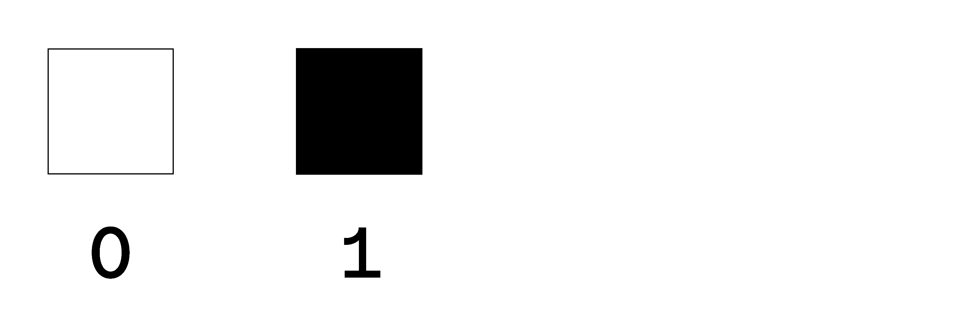
Now that the number of modules \(n=2\) is fixed, we have to choose the class for our permutation space. With a fast calculation \(tot=2^k\) we can get an idea of how many nodes will be included in our system:
with two digits \(k=2\) we can obtain four nodes \(tot=2^2=4\),
00, 01, 10, 11.with three digits \(k=3\) we can obtain eight nodes \(tot=2^3=8\),
000, 001, 010, 011, 100, 101, 110, 111.with four digits \(k=4\) we can obtain eight nodes \(tot=2^4=16\),
0000, 0001, 0010, 0011, 0100, 0101, 0110, 0111,
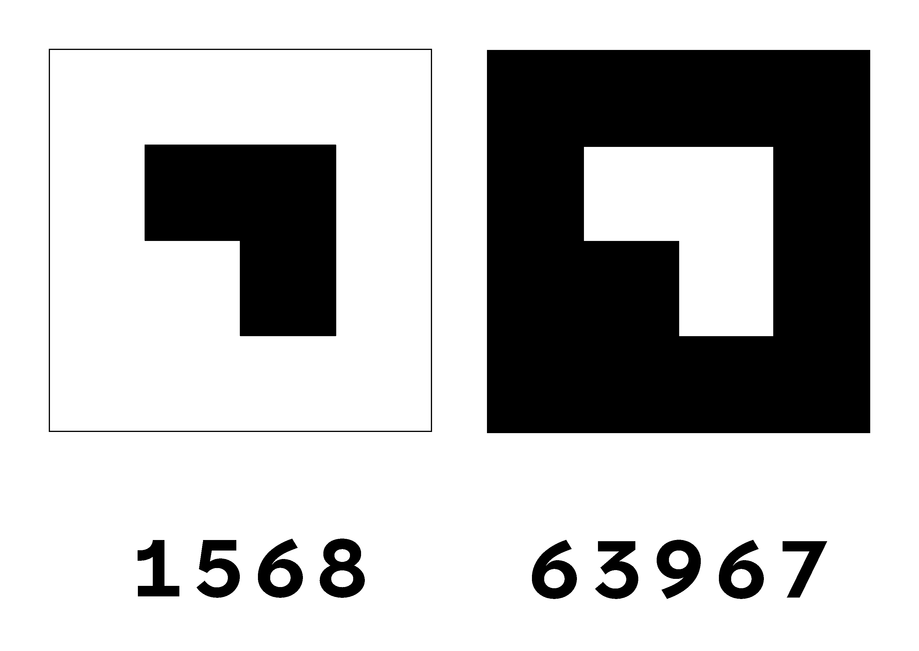
1000, 1001, 1010, 1011, 1100, 1101, 1110, 1111.It is clear that some values for k are more useful to us than others: the approrpiately-named perfect squares. Integers that can be actually arranged to form a square matrix. In order to obtain a decorative system complex enough we will use sixteen digits \(k=16\), obtaining a total of \(tot= 2^{16}=65.536\) nodes. This class allows as to format the strings of length 16 as 4x4 square matrices.
e.g. number 31828 is binary string
0111110001010100, which can be folded into the following
square matrix (using conventional top-down left-right folding):
31828  →  0111 1100 0101 0100  →  0 1 1 1
                                  1 1 0 0
                                  0 1 0 1
                                  0 1 0 0
Figure 16: Folding of a binary string into a square matrix.
After we have fixed our generation space to two modules \(n=2\) and sixteen digits \(k=16\) we can tell that we will obtain \(65.536\) nodes. In order to generate them, all we have to do is to count from 0 to 65.535 and convert the base of the numbers from 10 to 2.
We have now obtained 65.536 nodes (binary strings) of 16 digits, composed of 0 and 1.
0000000000000000, 0000000000000001,
0000000000000010, 0000000000000011,
0000000000000100, 0000000000000101
              ... 1111111111111111.
These can be folded to square matrices accordingly:
0 0 0 0   0 0 0 0   0 0 0 0   ...   1 1 1 1
0 0 0 0   0 0 0 0   0 0 0 0         1 1 1 1
0 0 0 0   0 0 0 0   0 0 0 0         1 1 1 1
0 0 0 0   0 0 0 1   0 0 1 0         1 1 1 1
This set includes all the possible nodes that can be created with these two modules with sixteen digits. Every resulting pattern is different from the other by at least one element.
The number 2025
0000111111001001,2025 → 0000 1111 1100 1001 → 0 0 0 0 → □ □ □ □
1 1 1 1 ■ ■ ■ ■
1 1 0 0 ■ ■ □ □
1 0 0 1 ■ □ □ ■Figure 17: Converting a decimal number to a 4x4 matrix.
Following the Truchet approach we now need to index the strings following some criterias. The indexing strictly depends on the purposes of our generative system. If we are going to produce visual patterns, we would want to catalogue nodes based on their visual appearance. In our case 0 and 1 represent a white or black square.
If for instance we consider the nodes obtained as rhythms (0 as silence and 1 as a specific sound), we should index them with different criterias that have more to do with music, rather than visual arts.
In order to demonstrate the improvement of Doüat’s notation we keep working on visual patterns, but this time we work with 4x4 square nodes, rather than 16x1 string nodes like Doüat. This will allow us to introduce a new kind of criteria for indexing, based on the symmetries of a square.
Doüat performs combinatorial calculation and enumerates the results obtained from \(1\) to \(n^k\). We want to keep naming nodes in decimal notation as it is the most common way to refer to integer numbers. We have also seen that expressing nodes in the natural base, the one that has the selected number of different digits presents many advantages: in the natural base the node Identifier coincides with the node description itself. To uniquely relate decimal representations to base-n strings one can use the base-change transformation, which maintains a one-to-one corispondence without error.
In the case of two modules: - we select 𝑛=2 modules and pick a perfect square class, say \(k=16\) - we count the total possible nodes as \(2^{16}\), from \(0\) to \(65,535\), this decimal number is the node identifier. - we convert to the natural binary base, this is the descriptive string for the node. - we can use this string for visually represent the node in a \(4×4\) grid.
Using decimal literals as identifiers for compositions poses a problem of long non-descriptive identifier: if we are navigating in a generative system with a large class, it may have so many elements that they have a long name, even if the modules of the system are only two. :::info I.e.
n = 2
k = 36
The node’s decimal ID number is:
18.345.642.073.719.551.315Even if it is shorter than its description in binary notation:
1111111010011000110100000100010001000100100000111011010101010011it results distant from day-to-day numbers. :::
Another limit consists in having a number of modules bigger than 10 (\(n>10\)). In this case the default base-10 identifier of a node would be longer than its “description”. It would be paradoxically easier to call a node by its description rather than its identifier.
I.e.
n = 16
k = 8
The node’s ID is:
10.268.320and its representation in hexadecimal notation is:
FAB10From the total set of nodes we can select a few with analogue visual properties.
Compositions can be indexed, for example, according to the count of total 0 and 1 digits. If 0 is white and 1 is black, this type of indexing corresponds to the average gray value of the composition. #### Indexing based on chromatic opposition This type of indexing leads to a further subdivision: for each composition there exists another in which the 0s and 1s are inverted (fig. 18). This allows us to divide the set into two symmetric parts: for any node with \(ID = t\) (where \(t\) is a decimal number), there exists its chromatic complement \(invID = n^k–t-1\) (where the \(n\) is the number of modules, and \(k\) is the class of the permutation).
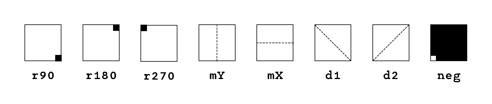
Each square node possesses 7 geometric symmetries (fig. 19): three rotations (90°, 180°, 270°) and four axial symmetries, corresponding to reflections along the vertical axis, the horizontal axis, and the two diagonals. In addition to these geometric symmetries, in a binary system we consider the inversion of 0 and 1 as a chromatic (or complementary) symmetry. This chromatic inversion is analogous to swapping black and white in the node’s configuration, resulting in what we call the complementary node.
As a consequence, each node is associated with a total of 16 related nodes: 8 obtained by applying the 7 geometric symmetries and the original configuration, 8 more by applying the same symmetries to its chromatic complement. This is why nodes are grouped in sets of 16: each set contains a node, all its geometric symmetries, its chromatic complement, and all the symmetries of the complement (fig. 20).
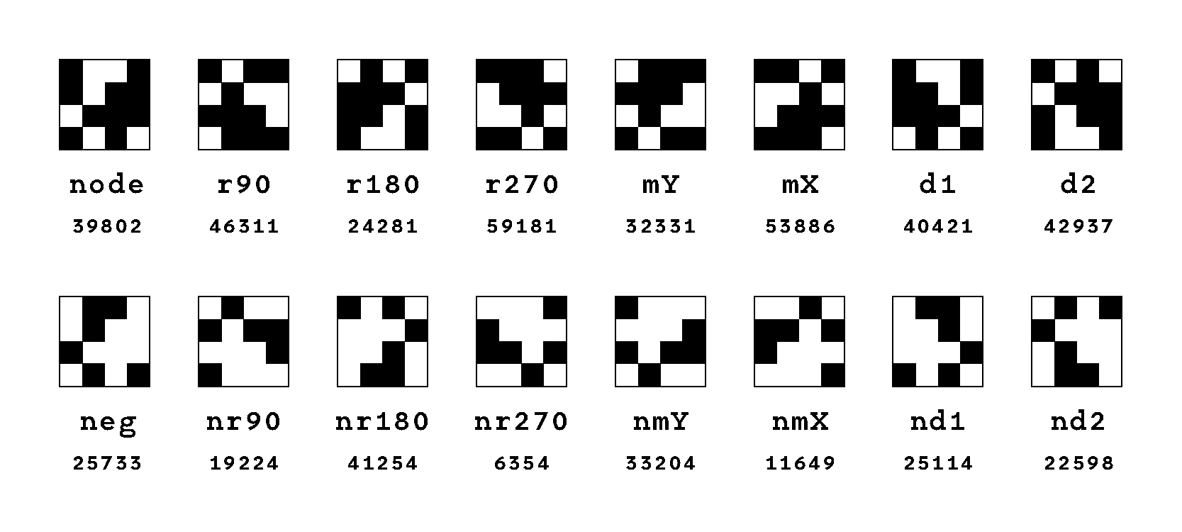
Interestingly, not all nodes are unique under these transformations. Some nodes are invariant under certain symmetries; for example, a node that is symmetric with respect to the vertical axis remains unchanged when reflected along that axis (fig. 21).
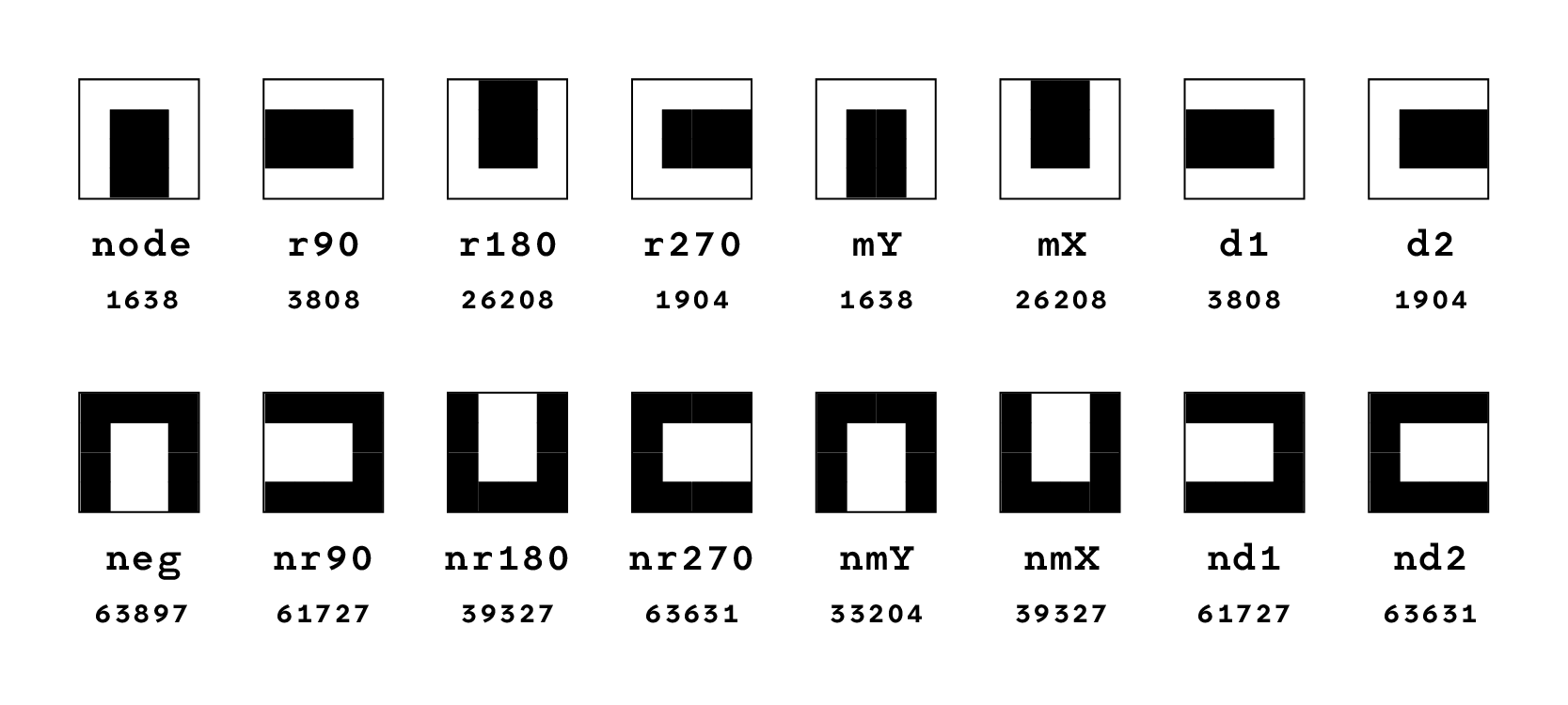
This redundancy creates a simplification: some of the 16 transformations may yield the same node, reducing the actual number of distinct nodes in the resulting set (fig. 22).
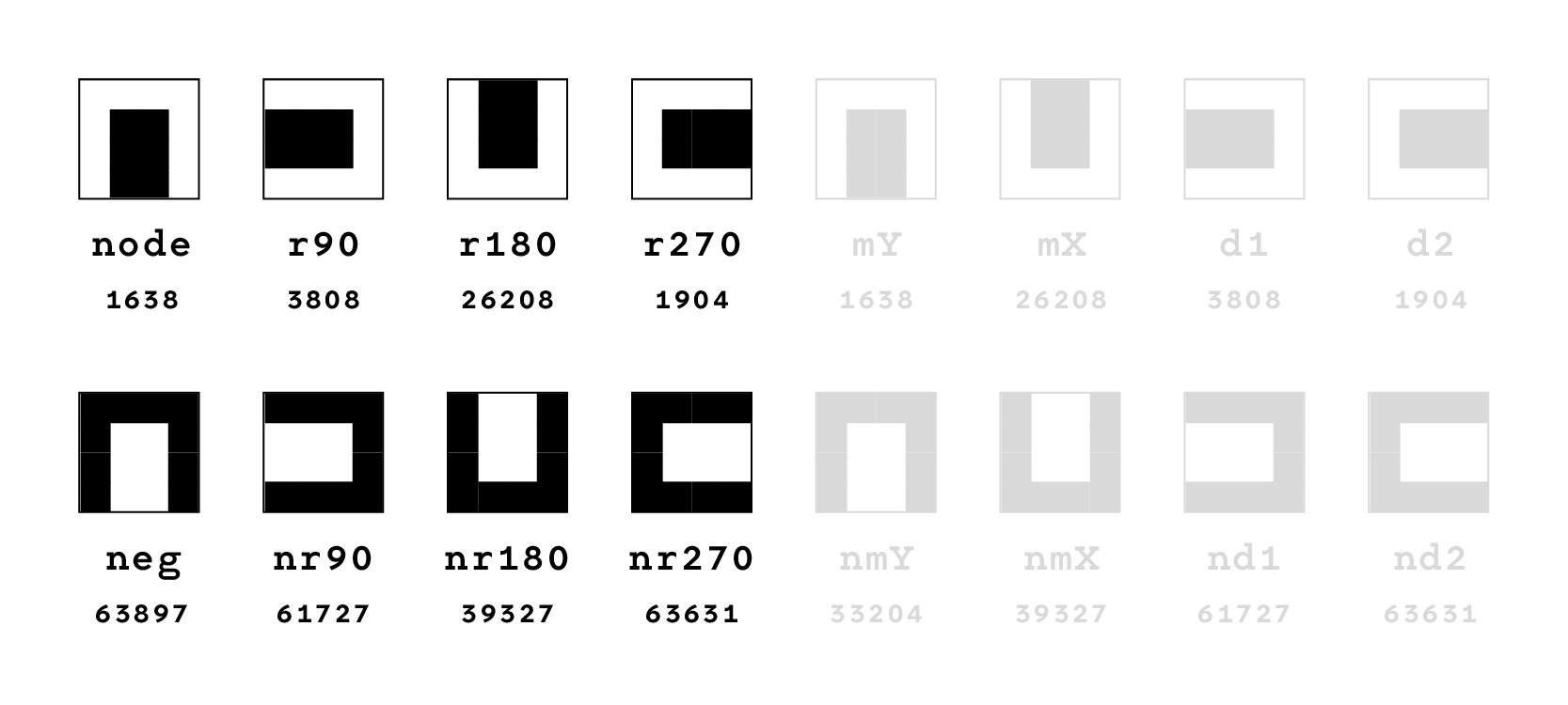
Indexing nodes according to the type and number of redundant symmetries provides a powerful way to classify them. Nodes with the same redundancy profile share common geometric or chromatic properties, which can be useful for analyzing, selecting specific nodes, or generating patterns within the larger system. An example of this classification can be found in the appendix B.
Dominique Doüat described and used some generative rules for creating tilings (“desseins”) by selecting specific permutations from a comprehensive table of all possible combinations of tiles. These rules determine which permutations to choose, how to arrange them, and how to repeat these arrangements. By carefully choosing, positioning, and combining these permutations according to set procedures, Doüat’s approach enables the creation of a wide variety of increasingly complex designs through clear, repeatable steps.
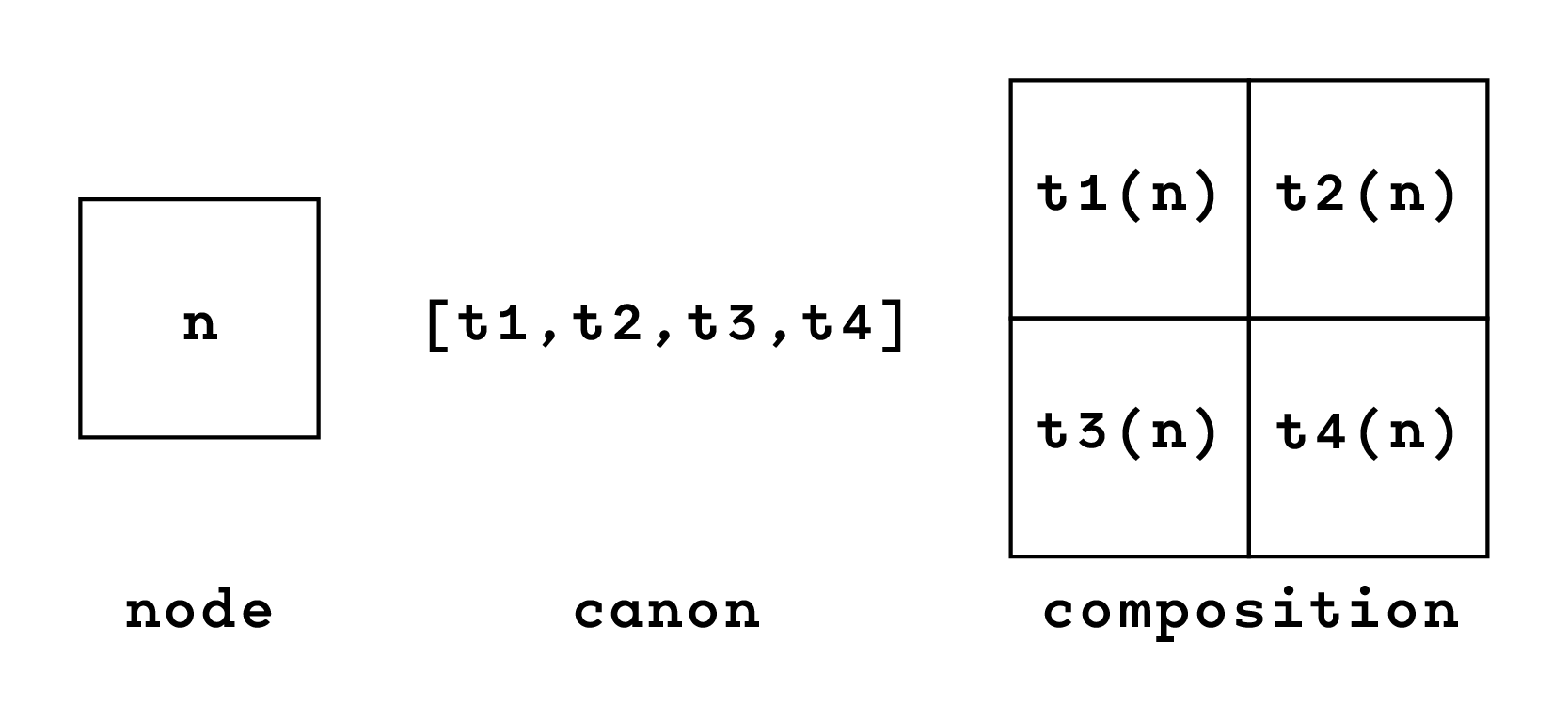
We refer to this kind of rules with the word “canon”, as a “set of transformations”, a list of operations to execute on the node to produce a larger composition. By working on a square grid we know that combining four adjacent modules in a 2x2 format produces a larger square composition (fig. 23).
//Rotations
r90   //90 degree rotation
r180  //180 degree rotation
r270  //270 degree rotation

//Reflections
mX  //reflection on the X axis
mY  //reflection on the Y axis
d1  //reflection on the first diagonal
d2  //reflection on the second diagonal

//Chromatic inversion
ne  //inversion of "0" and "1"
Figure 24: Complete list of transformations with their short name.
In terms of canon notation the order of the sequence always starts from the upper left corner, and follows to the right, then repeats on the new line. This is done to stay coherent to the typographic approach and ensure the same flow of information between nodes, canons, and compositions.
notation = [n1,n2,n3,n4] = ⎡n1,n2⎤
                           ⎣n3,n4⎦


rep = [n,n,n,n] // Repetition

nRep = [ne,ne,ne,ne] // Negative repetition
altRep = [n,ne,ne,n] // Alternated repetition

refX = [n,n,mX,mX] // Horizontal mirror
refY = [n,mY,n,mY] // Vertical mirror
refD = [n,d2,d2,n] // Diagonal mirror

altRefX = [ne,ne,mX,mX] // Alt. horizontal mirror
altRefY = [n,ne(mY),n,ne(mY)] // Alt. vertical mirror
altRefD = [n,ne(d2),ne(d2),n] // Alt. diagonal mirror

ortho = [n,mY,mX,r180] // Orthogonal
altOrtho = [n,ne(mY),ne(mX),r180] // Alternate orthogonal

rotC = [n,r90,r270,r180] // Concentric rotation
altRotC = [ne,ne(r90),ne(r270),ne(r180)] // Neg. conc. rotation
Figure 26: A complete list of the syntax of the canons
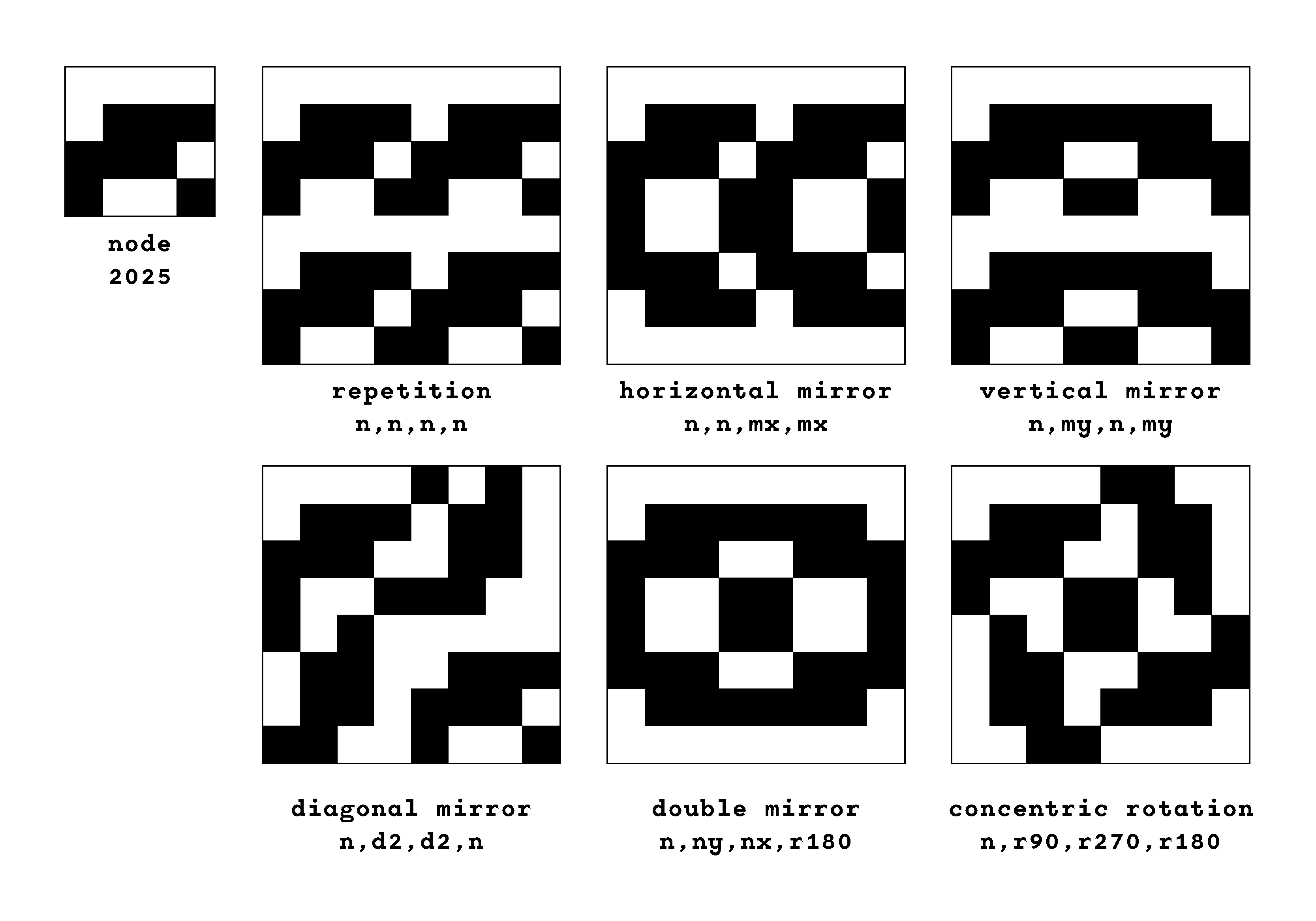
Founding the system on a power of four principle opens up to many possibilities. By applying a canon to a node, we obtain a composition that is still a perfect square (fig. 28). Therefore, treating the result composition as an input node, we can pass it through a second canon (fig. 29) and repeat the process to get another perfect square. The canon operation exhibits the inherent property of nesting: we can travel through “layers” of canons, increasing the complexity of the resulting composition and its resolution. (fig. 30)
It is important to note that commutative property does not apply to canon nesting: the same canons applied to the node in different order can produce a different composition.
We invite the reader to explore canon nesting in the Chicken Counter tool that we present in Appendix A. It is focused on intuitive exploration of the node symmetries and composition of 3 layers of canons, applied to a manually designed 4x4 node.
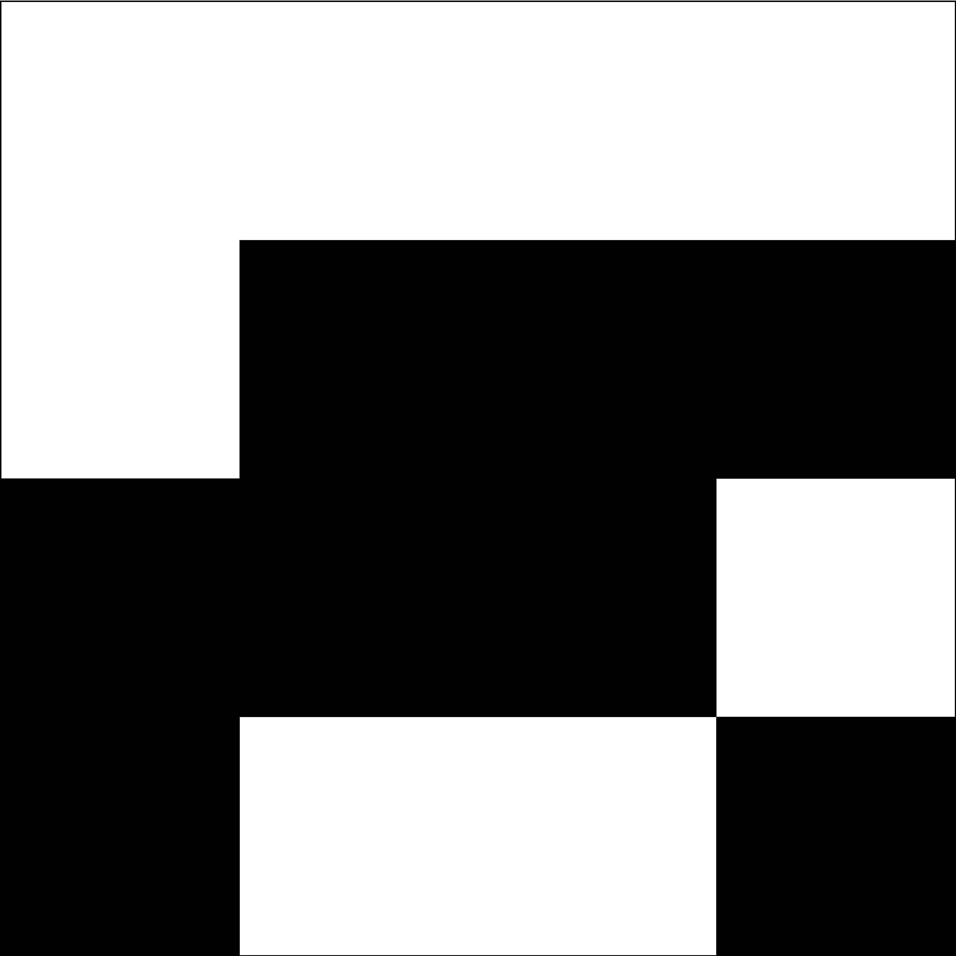
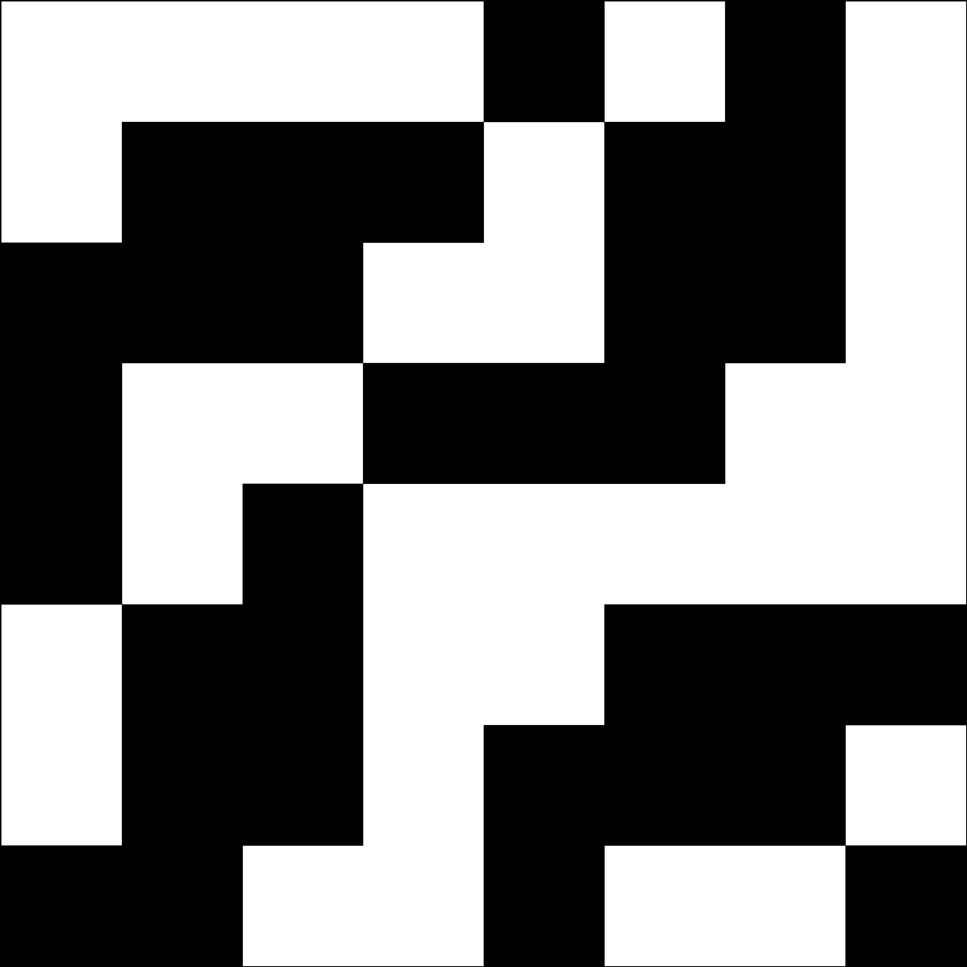
![Figure 29: Pattern obtained with doubleMirror[diagonalMirror(2025)]](media/9ddc6c683a5d9f5766e867a559f16e1573cebffe.png)
![Figure 30: Pattern obtained with repetition{doubleMirror[diagonalMirror(2025)]}](media/4a3249f1765483e15ef9e1c60820a7606ec17768.png)
This paper has demonstrated how Dominique Doüat’s combinatorial notation can be adapted for computational pattern generation by reframing visual compositions as numeric literals in a positional counting system. By treating Doüat’s combinatorial strings as base-n numbers, we have transformed the manual enumeration process into efficient computational counting, enabling the systematic generation and analysis of all possible pattern combinations within parameter spaces defined by number of different modules and class.
Our approach centers on grouping enumerated elements into coherent sets based on structural properties — particularly symmetry redundancies — which provides a powerful framework for pattern classification and selection. This mathematical foundation honors Doüat’s 18th-century innovations and extends them into contemporary computational practice, revealing new affordances for pattern exploration and generation.
The efficiency gains from treating patterns as numeric literals rather than character strings prove substantial. Operating directly on numbers allows for rapid generation, comparison, and manipulation of entire pattern spaces—transformations that would be computationally expensive when performed on string representations. This numeric approach enables real-time exploration of pattern sets containing tens of thousands of elements, making previously impractical systematic analysis feasible.
Critically, our method reconciles two seemingly conflicting creative approaches. The bottom-up approach begins with mathematical enumeration, building pattern understanding through systematic analysis of all possible combinations and their structural properties, then filtering based on them. Conversely, the top-down approach starts with intuitive exploration, allowing designers to navigate the pattern space guided by aesthetic preference and creative intention. Rather than opposing each other, these approaches prove complementary: systematic enumeration provides the comprehensive foundation that makes intuitive exploration meaningful, while creative navigation reveals which mathematical structures hold visual or functional significance. The filtering and grouping mechanisms serve as the bridge between these approaches, transforming exhaustive mathematical coverage into selective creative discovery.
Free exploration has revealed symmetries emerging from computational analysis rather than traditional geometric classification. Visual analysis of contiguous shapes within patterns and mathematical characterization of node filters require further work. The approach may find application in musical composition and typography, though domain –specific constraints would need consideration.
The companion web application and playground “The Chicken Counter” provides a foundation for further exploration. Taken as a framework, it also opens the possibility of new curated functions to be implemented, leveraging simple interactions for a cascade of effects. Notably, the translation function within the nodes has revealed the potential to generate “organic” animations, evoking patterns reminiscent of Conway’s Game of Life.9.
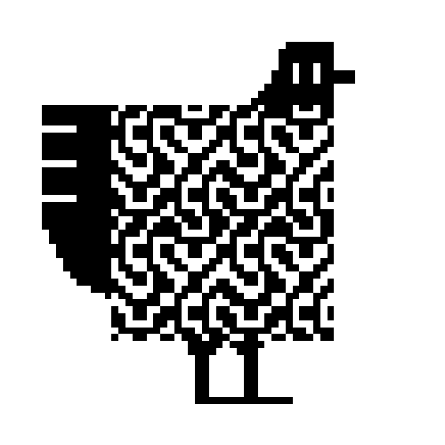
With 65,536 chickens scratching in a coop, how can one properly distinguish and move them around?
This paper comes with a companion web app allowing for free exploration of patterns: The Chicken Counter 1.0 is a browser-based interface to navigate the nodes (chickens) and arrange them into more advanced compositions.
It has been designed pursuing the smoothness of interaction. It is meant to be explored intuitively. It works as a playground, we invite you to explore it freely or to start from the selected nodes you encountered in the paper.
The primary parameters of our proposed method have been intentionally fixed for ease of use, and to reduce the complexity of the process to the lowest terms.
The core system of the counter is the decimal number, the unique identifier of each node-chicken (from 0 to 65,535). In this generator we display all the forms a node can take in our system: as a number, as binary strings (graphical or numerical), as binary matrices (graphical or numerical).
Since the number and the strings evade our human ability to graphically evaluate the corresponding node, we arranged the matrices representations at the top of the page. There they serve as the first interactive entry point. Each digit can be clicked and swapped to the opposed binary one, for an extremely intuitive and fast optical-based navigation of the nodes, while live-adjusting the underlying decimal indexing to always point to the correct value.
Whichever node selection route is taken, number or click based, the system responsively updates the others to always be in sync and display the correct decimal and binary representations.
The process so far has established a system to encode, identify and distinguish a precise amount of binary nodes. These nodes, strings of 16 characters, can be represented graphically, by employing a custom typeface that converts 1s to black squares and 0s to white ones.
A note on this choice: despite the semantic representation of 0 as black and 1 as white, we preferred to swap it graphically in order to represent the 1 as “presence of something” and “fullness” with the black square, against the “absence of something” and “emptiness” of the 0.
Our wish is to explore the graphical applications of the modules in a controlled environment, one that can enable us to navigate smoothly through the entire set of possibilities. All of this while maintaining a formal description of each resulting output.
Lastly, any users wishing to make concrete use of their exploration are welcome to copy the output, and incorporate it into whichever medium of interest they may have. Given the simple binary nature of the output, it may find applications from typography to punchcard for textiles, classic decoration or more advanced computational elaboration.
When we open the Chicken Counter and at every refresh we visualise a 32x32 composition, obtained through the nesting of three random canons, applied to a random node (chicken).
As a general rule, any red element is interactive, with the addition of the two matrices on the top right - in binary squares and digits.
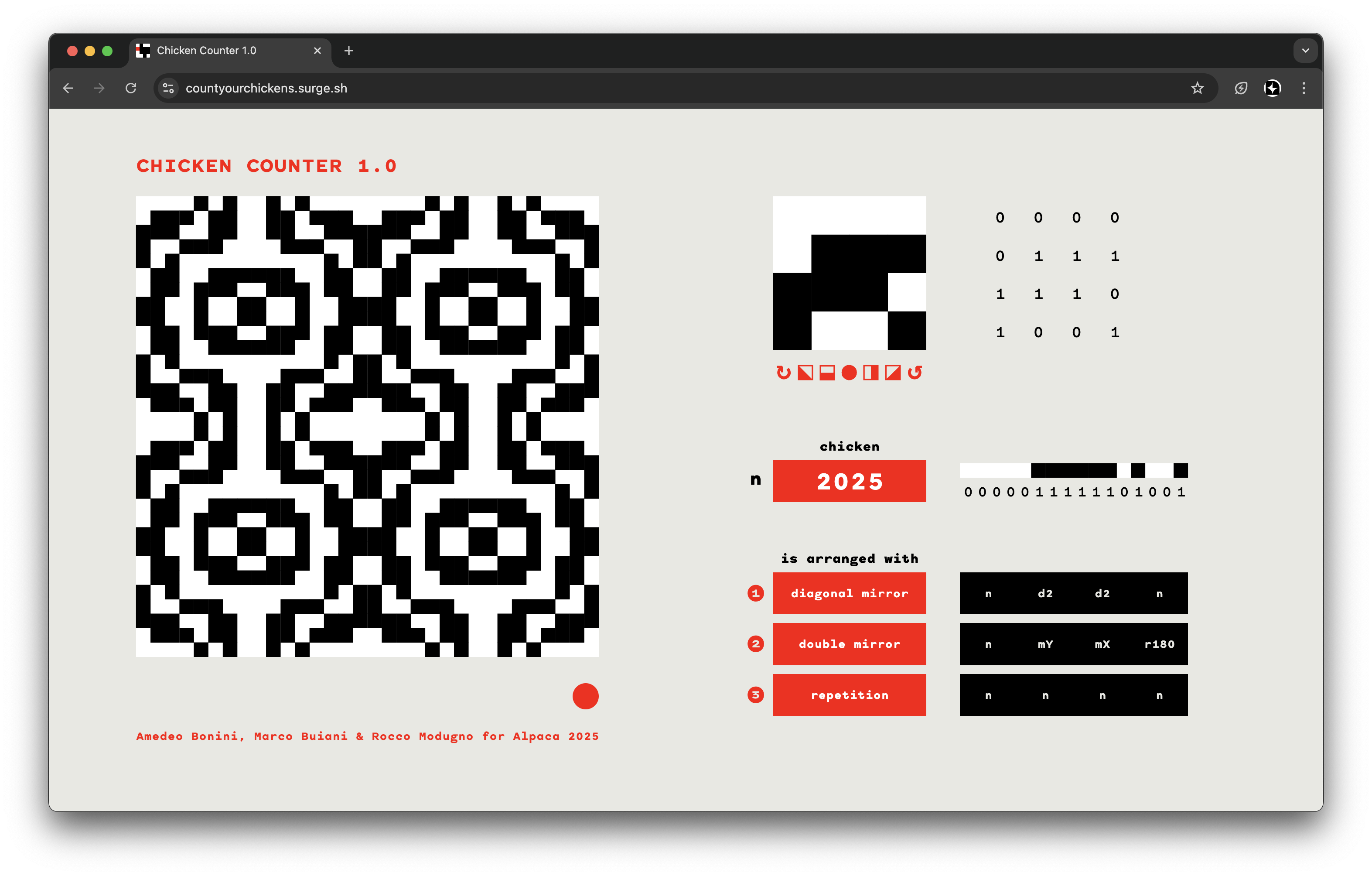
The controls are set to the right side of the window, here we can edit the nodes and the canons of the output composition.
The core system of the counter is the number, the unique identifier of each node-chicken. This univocal value is represented five times (fig. A2):
2025,□□□□□■■■■■■□■□□■,0000011111101001.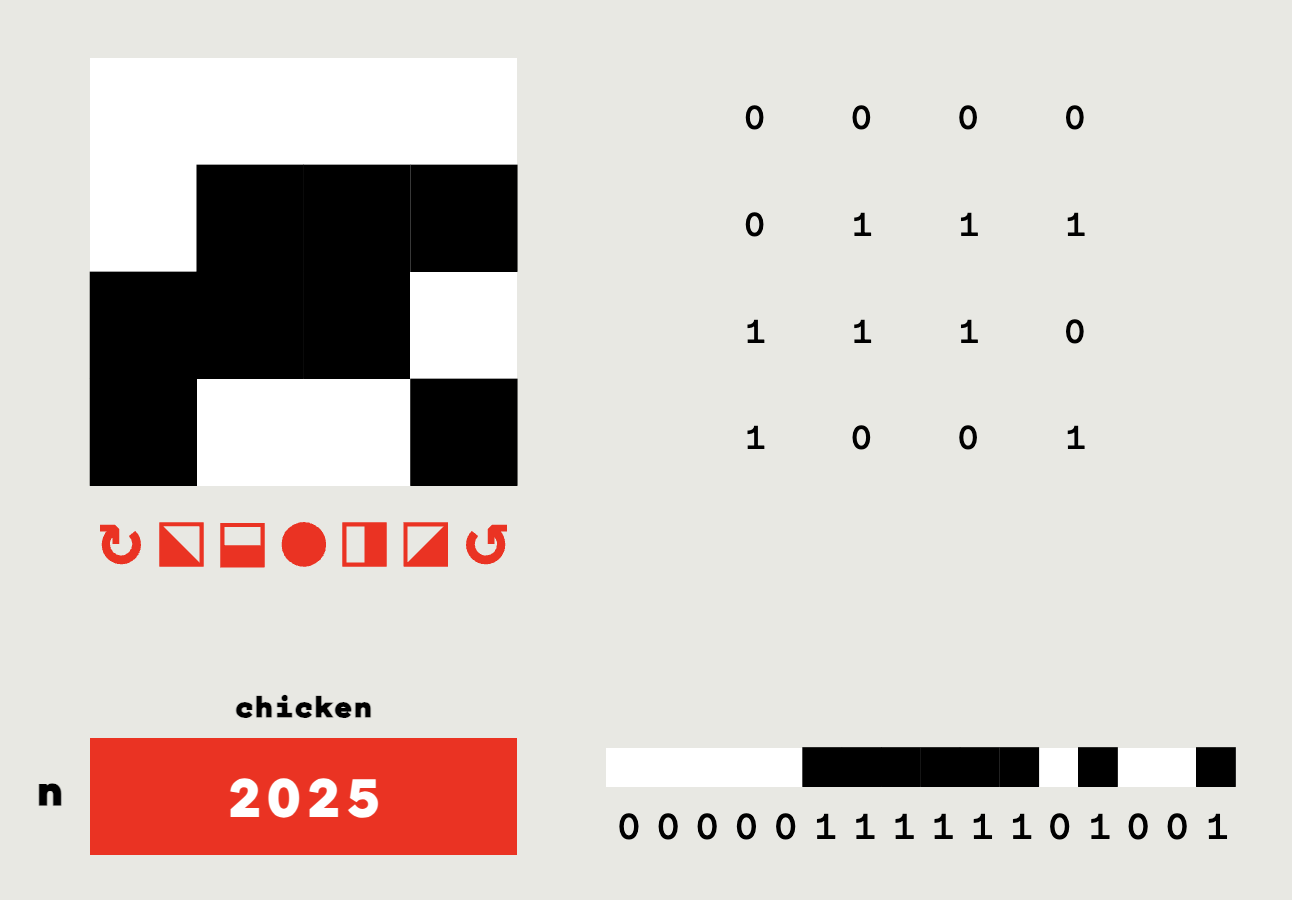
Both the matrices can have each individual digit clicked to swap it to the other binary value. Additionally, a transformation bar is located under the first matrix (fig. A3). Its different buttons apply the corresponding transformation to the module. From left to right, these are: 1. clockwise rotation, 2. first diagonal symmetry, 3. reflection on the horizontal axis, 4. complementary (negative), 5. reflection across vertical axis, 6. second diagonal symmetry, 7. and counterclockwise rotation.

An ulterior tool appears when hovering the square matrix (fig. A4). Four arrows pointing to its different sides, that upon being clicked shift the pattern a column or row up or down, depending on the direction clicked.
Under the node matrices is the Chicken Number, a decimal number input ranging from 0 to 65535, covering all the possible permutations of the class-16 binary module (fig. A5). Once clicked, a new number can be typed in or scrolled to using the up and down arrow keys. By clicking on the round button below, the chicken-number is randomized. On the right the node is represented both as a visual and numeric binary string.
The canons define the arrangement of the node in the larger compositions, they are randomly selected at page loading or by clicking on the title (fig. A6). A maximum nesting of three canons is allowed on the generator. On the right of each canon a black box displays the list of the transformations applied to the node. Canons are activated by default, and can be deactivated by clicking on their letter identifier (the red ❶, ❷ and ❸). By hovering the mouse over the red rectangular buttons, small arrows appears, they can be used to edit the applied canons. Furthermore, clicking on the round red button the canons are randomised.
The pattern preview is visible on the left side of the window. The output is read-only, and its content can be copied to the clipboard by clicking the red dot under the bottom-right corner (fig. A7).
It is a string of 1s and 0s separated into lines by carriage returns. You can render this text on any text editor whit this simple font, that displays 1s as black squares ■, and 0s as white ones □. Make sure to give the same value of body size and baseline, so that the squares align exactly.
00001010010100000000101001010000
01110110011011100111011001101110
11100110011001111110011001100111
10011100001110011001110000111001
10100000000001011010000000000101
01100111111001100110011111100110
01101110011101100110111001110110
11001001100100111100100110010011
11001001100100111100100110010011
01101110011101100110111001110110
01100111111001100110011111100110
10100000000001011010000000000101
10011100001110011001110000111001
11100110011001111110011001100111
01110110011011100111011001101110
00001010010100000000101001010000
00001010010100000000101001010000
01110110011011100111011001101110
11100110011001111110011001100111
10011100001110011001110000111001
10100000000001011010000000000101
01100111111001100110011111100110
01101110011101100110111001110110
11001001100100111100100110010011
11001001100100111100100110010011
01101110011101100110111001110110
01100111111001100110011111100110
10100000000001011010000000000101
10011100001110011001110000111001
11100110011001111110011001100111
01110110011011100111011001101110
00001010010100000000101001010000
Figure 38: Output of the Chicken Counter 1.0, using the node 2025 and applying the diagonal mirror, double mirror, and repetition canons.
Once all possible nodes have been indexed, it becomes easy to isolate those with specific structural properties by applying filtering rules.
Dichromatic symmetry identifies the graphical elements made of only two colors in which the shape of one color and the shape of the chromatic opposite are complementary and identical in shape;
A famous example is the Yin and Yang symbol.
Nodes for which at least one of the fundamental square transformations produces the chromatic inverse are of this kind.
One can reproduce this process as follows: 1. select nodes that are half black, those with the same number of zeroes and ones; 2. apply the 7 square transformations and mark the results; 3. compare each result with the inverse of the original: if one or more matches you got one.
All possible permutations can be filtered to extract compositions with particularly distinctive properties, enabling the abstraction and study of modules that exhibit notable formal or perceptual characteristics.
We further group them in closed sets by the number of unique results after symmetries.
 Figure B1: 100 Pixel nodes with dichromatic
symmetry in a square matrix of class 16.
Figure B1: 100 Pixel nodes with dichromatic
symmetry in a square matrix of class 16.
| Class 10 Numeral String | Class 4 Numeral with Leading 0s | Doüat Notation |
|---|---|---|
| 0 | 0000 | AAAA |
| 1 | 0001 | AAAB |
| 2 | 0002 | AAAC |
| 3 | 0003 | AAAD |
| 4 | 0010 | AABA |
| 5 | 0011 | AABB |
| 6 | 0012 | AABC |
| 7 | 0013 | AABD |
| 8 | 0020 | AACA |
| 9 | 0021 | AACB |
| 10 | 0022 | AACC |
| 11 | 0023 | AACD |
| 12 | 0030 | AADA |
| 13 | 0031 | AADB |
| 14 | 0032 | AADC |
| 15 | 0033 | AADD |
| 16 | 0100 | ABAA |
| 17 | 0101 | ABAB |
| 18 | 0102 | ABAC |
| 19 | 0103 | ABAD |
| 20 | 0110 | ABBA |
| 21 | 0111 | ABBB |
| 22 | 0112 | ABBC |
| 23 | 0113 | ABBD |
| 24 | 0120 | ABCA |
| 25 | 0121 | ABCB |
| 26 | 0122 | ABCC |
| 27 | 0123 | ABCD |
| 28 | 0130 | ABDA |
| 29 | 0131 | ABDB |
| 30 | 0132 | ABDC |
| 31 | 0133 | ABDD |
| 32 | 0200 | ACAA |
| 33 | 0201 | ACAB |
| 34 | 0202 | ACAC |
| 35 | 0203 | ACAD |
| 36 | 0210 | ACBA |
| 37 | 0211 | ACBB |
| 38 | 0212 | ACBC |
| 39 | 0213 | ACBD |
| 40 | 0220 | ACCA |
| 41 | 0221 | ACCB |
| 42 | 0222 | ACCC |
| 43 | 0223 | ACCD |
| 44 | 0230 | ACDA |
| 45 | 0231 | ACDB |
| 46 | 0232 | ACDC |
| 47 | 0233 | ACDD |
| 48 | 0300 | ADAA |
| 49 | 0301 | ADAB |
| 50 | 0302 | ADAC |
| 51 | 0303 | ADAD |
| 52 | 0310 | ADBA |
| 53 | 0311 | ADBB |
| 54 | 0312 | ADBC |
| 55 | 0313 | ADBD |
| 56 | 0320 | ADCA |
| 57 | 0321 | ADCB |
| 58 | 0322 | ADCC |
| 59 | 0323 | ADCD |
| 60 | 0330 | ADDA |
| 61 | 0331 | ADDB |
| 62 | 0332 | ADDC |
| 63 | 0333 | ADDD |
| 64 | 1000 | BAAA |
| 65 | 1001 | BAAB |
| 66 | 1002 | BAAC |
| 67 | 1003 | BAAD |
| 68 | 1010 | BABA |
| 69 | 1011 | BABB |
| 70 | 1012 | BABC |
| 71 | 1013 | BABD |
| 72 | 1020 | BACA |
| 73 | 1021 | BACB |
| 74 | 1022 | BACC |
| 75 | 1023 | BACD |
| 76 | 1030 | BADA |
| 77 | 1031 | BADB |
| 78 | 1032 | BADC |
| 79 | 1033 | BADD |
| 80 | 1100 | BBAA |
| 81 | 1101 | BBAB |
| 82 | 1102 | BBAC |
| 83 | 1103 | BBAD |
| 84 | 1110 | BBBA |
| 85 | 1111 | BBBB |
| 86 | 1112 | BBBC |
| 87 | 1113 | BBBD |
| 88 | 1120 | BBCA |
| 89 | 1121 | BBCB |
| 90 | 1122 | BBCC |
| 91 | 1123 | BBCD |
| 92 | 1130 | BBDA |
| 93 | 1131 | BBDB |
| 94 | 1132 | BBDC |
| 95 | 1133 | BBDD |
| 96 | 1200 | BCAA |
| 97 | 1201 | BCAB |
| 98 | 1202 | BCAC |
| 99 | 1203 | BCAD |
| 100 | 1210 | BCBA |
| 101 | 1211 | BCBB |
| 102 | 1212 | BCBC |
| 103 | 1213 | BCBD |
| 104 | 1220 | BCCA |
| 105 | 1221 | BCCB |
| 106 | 1222 | BCCC |
| 107 | 1223 | BCCD |
| 108 | 1230 | BCDA |
| 109 | 1231 | BCDB |
| 110 | 1232 | BCDC |
| 111 | 1233 | BCDD |
| 112 | 1300 | BDAA |
| 113 | 1301 | BDAB |
| 114 | 1302 | BDAC |
| 115 | 1303 | BDAD |
| 116 | 1310 | BDBA |
| 117 | 1311 | BDBB |
| 118 | 1312 | BDBC |
| 119 | 1313 | BDBD |
| 120 | 1320 | BDCA |
| 121 | 1321 | BDCB |
| 122 | 1322 | BDCC |
| 123 | 1323 | BDCD |
| 124 | 1330 | BDDA |
| 125 | 1331 | BDDB |
| 126 | 1332 | BDDC |
| 127 | 1333 | BDDD |
| 128 | 2000 | CAAA |
| 129 | 2001 | CAAB |
| 130 | 2002 | CAAC |
| 131 | 2003 | CAAD |
| 132 | 2010 | CABA |
| 133 | 2011 | CABB |
| 134 | 2012 | CABC |
| 135 | 2013 | CABD |
| 136 | 2020 | CACA |
| 137 | 2021 | CACB |
| 138 | 2022 | CACC |
| 139 | 2023 | CACD |
| 140 | 2030 | CADA |
| 141 | 2031 | CADB |
| 142 | 2032 | CADC |
| 143 | 2033 | CADD |
| 144 | 2100 | CBAA |
| 145 | 2101 | CBAB |
| 146 | 2102 | CBAC |
| 147 | 2103 | CBAD |
| 148 | 2110 | CBBA |
| 149 | 2111 | CBBB |
| 150 | 2112 | CBBC |
| 151 | 2113 | CBBD |
| 152 | 2120 | CBCA |
| 153 | 2121 | CBCB |
| 154 | 2122 | CBCC |
| 155 | 2123 | CBCD |
| 156 | 2130 | CBDA |
| 157 | 2131 | CBDB |
| 158 | 2132 | CBDC |
| 159 | 2133 | CBDD |
| 160 | 2200 | CCAA |
| 161 | 2201 | CCAB |
| 162 | 2202 | CCAC |
| 163 | 2203 | CCAD |
| 164 | 2210 | CCBA |
| 165 | 2211 | CCBB |
| 166 | 2212 | CCBC |
| 167 | 2213 | CCBD |
| 168 | 2220 | CCCA |
| 169 | 2221 | CCCB |
| 170 | 2222 | CCCC |
| 171 | 2223 | CCCD |
| 172 | 2230 | CCDA |
| 173 | 2231 | CCDB |
| 174 | 2232 | CCDC |
| 175 | 2233 | CCDD |
| 176 | 2300 | CDAA |
| 177 | 2301 | CDAB |
| 178 | 2302 | CDAC |
| 179 | 2303 | CDAD |
| 180 | 2310 | CDBA |
| 181 | 2311 | CDBB |
| 182 | 2312 | CDBC |
| 183 | 2313 | CDBD |
| 184 | 2320 | CDCA |
| 185 | 2321 | CDCB |
| 186 | 2322 | CDCC |
| 187 | 2323 | CDCD |
| 188 | 2330 | CDDA |
| 189 | 2331 | CDDB |
| 190 | 2332 | CDDC |
| 191 | 2333 | CDDD |
| 192 | 3000 | DAAA |
| 193 | 3001 | DAAB |
| 194 | 3002 | DAAC |
| 195 | 3003 | DAAD |
| 196 | 3010 | DABA |
| 197 | 3011 | DABB |
| 198 | 3012 | DABC |
| 199 | 3013 | DABD |
| 200 | 3020 | DACA |
| 201 | 3021 | DACB |
| 202 | 3022 | DACC |
| 203 | 3023 | DACD |
| 204 | 3030 | DADA |
| 205 | 3031 | DADB |
| 206 | 3032 | DADC |
| 207 | 3033 | DADD |
| 208 | 3100 | DBAA |
| 209 | 3101 | DBAB |
| 210 | 3102 | DBAC |
| 211 | 3103 | DBAD |
| 212 | 3110 | DBBA |
| 213 | 3111 | DBBB |
| 214 | 3112 | DBBC |
| 215 | 3113 | DBBD |
| 216 | 3120 | DBCA |
| 217 | 3121 | DBCB |
| 218 | 3122 | DBCC |
| 219 | 3123 | DBCD |
| 220 | 3130 | DBDA |
| 221 | 3131 | DBDB |
| 222 | 3132 | DBDC |
| 223 | 3133 | DBDD |
| 224 | 3200 | DCAA |
| 225 | 3201 | DCAB |
| 226 | 3202 | DCAC |
| 227 | 3203 | DCAD |
| 228 | 3210 | DCBA |
| 229 | 3211 | DCBB |
| 230 | 3212 | DCBC |
| 231 | 3213 | DCBD |
| 232 | 3220 | DCCA |
| 233 | 3221 | DCCB |
| 234 | 3222 | DCCC |
| 235 | 3223 | DCCD |
| 236 | 3230 | DCDA |
| 237 | 3231 | DCDB |
| 238 | 3232 | DCDC |
| 239 | 3233 | DCDD |
| 240 | 3300 | DDAA |
| 241 | 3301 | DDAB |
| 242 | 3302 | DDAC |
| 243 | 3303 | DDAD |
| 244 | 3310 | DDBA |
| 245 | 3311 | DDBB |
| 246 | 3312 | DDBC |
| 247 | 3313 | DDBD |
| 248 | 3320 | DDCA |
| 249 | 3321 | DDCB |
| 250 | 3322 | DDCC |
| 251 | 3323 | DDCD |
| 252 | 3330 | DDDA |
| 253 | 3331 | DDDB |
| 254 | 3332 | DDDC |
| 255 | 3333 | DDDD |
The Chicken Counter 1.0 web app https://countyourchickens.surge.sh/↩︎
Sebastien Truchet, Memoire sur les combinations. Memoires de l’Academie Royale des sciences, Paris, 1704.↩︎
Dominique Doüat, Méthode pour faire une infinité de desseins différents avec des carreaux mi-partis de deux couleurs par une ligne diagonale : ou observations du Père Dominique Doüat, Religieux Carme de la Province de Toulouse, sur un mémoire inséré dans l’Histoire de l’Académie Royale des Sciences de Paris l’année 1704, présenté par le Révérend Père Sébastien Truchet, religieux du même ordre, Académicien honoraire; Printed by Jacques Quillau, Paris, 1722.↩︎
Original text: Le même carreau A, étant diversement placé et aperçu d’un même côté, peut être regardé comme quatre différents carreaux: cela est clair. Nous appellerons carreau A celui qui a l’angle coloré en bas à main gauche; carreau B, celui qui a l’angle coloré en haut à main gauche; carreau C, celui qui a l’angle coloré en haut à main droite; et carreau D, celui qui a l’angle coloré en bas à main droite. Voyez la planche première, figure 2.↩︎
Douat (1722), pp. 18–19.↩︎
Lorenz, M. (2021). Flexible Visual Systems: A design manual for contemporary visual identities (B. Boyer & D. Marshall, Eds.). Slanted Publishers. ISBN 978‑3‑948440‑30‑5↩︎
https://www.lascuolaopensource.xyz/en/archivio/generatore-tipografico-di-liberta↩︎
Modugno, Rocco Lorenzo. 2023. “Tiling through Typography.” In Algorithmic Pattern Salon. Then Try This. https://doi.org/10.21428/108765d1.7ce0eb8b.↩︎
https://en.wikipedia.org/wiki/Conway%27s_Game_of_Life↩︎